

The methodology is illustrated in Fig. 2. The first section (left side) elucidates the methods, including vulnerability metrics, scaling method, vulnerability scoring formulation, and description of indicators used. The second section (right side) addresses the implementation of the model in a case, including data sources, data extraction, data transformation, vulnerability score computation, and reporting and analysis.
Fig. 2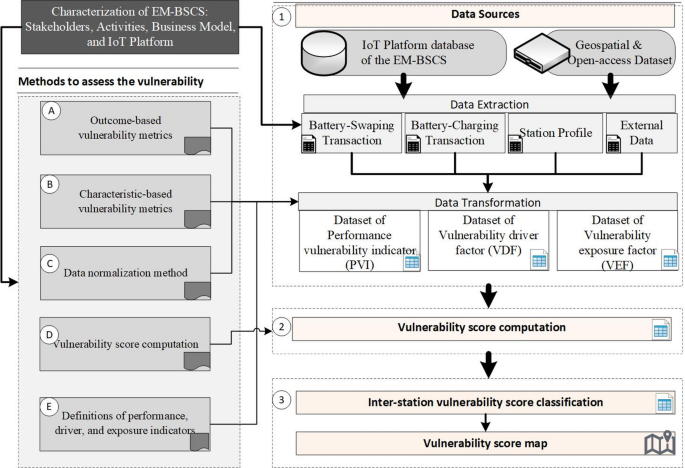
Methodology to develop vulnerability score on EM-BSCS.
Proposed vulnerability concept
Based on those vulnerability concepts in the previous subsection, there are two types of vulnerability impact: risk and performance degradation. The concept of vulnerability is proposed in Fig. 3. Vulnerability refers to a condition when performance falls outside the defined bounds of the expected range, driven by internal preconditions that may be weak in resisting exposure factors, which can themselves directly exacerbate performance degradation. Additionally, the system is vulnerable while performance remains outside the defined bounds, neither improving nor recovering, but instead continuing to deteriorate. This concept adopts performance measures as vulnerability impacts or system outcomes, as it is more readily observable in big data than risk-based measures. Both the magnitude and frequency of performance degradation serve as metrics for assessing vulnerability levels.
Fig. 3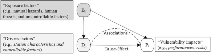
Vulnerability model in the EM-BSCS.
Internal preconditions are driver factors that refer to operational characteristics of the EM-BSCS, which represent the system’s mitigation ability and may drive an increase or decrease in the vulnerability impacts. For instance, the availability of cabinets and batteries at a station enhances mitigation capability, thereby reducing performance impacts like low battery swapping throughput. Similarly, fewer customers swapping batteries at SoC levels below the ideal threshold can minimize battery degradation, leading to greater diversity in battery circulation and higher swapping throughput. Ultimately, these internal precondition factors (driver factors) reflect system conditions that are within operational control.
Exposure factors are station characteristics that represent external influences or uncontrollable factors (e.g., natural hazards, human threats) that may exploit driver factors and intensify the impact of vulnerability (performance degradation). For example, flood risk at a station might hinder mitigation capability and degrade system performance. The quantity of operational failure modes in battery swapping could increase the swapping duration time and decrease the throughput levels. Likewise, higher customer engagement in battery charging services could reduce cabinet availability for battery swapping and decrease throughput levels.
Outcome-based vulnerability metrics
Outcome-based vulnerability metrics are measured through performance values. A system is considered vulnerable (VL = 1) at time t if the performance value \(x_t\) falls outside the defined bounds of the expected (robustness) range (see Eq. 1). Time \(t\) is the smallest period in which the performance value can be observed (e.g., hourly or daily), and \(T\) is the length of the observation time (e.g., a month). The bounds, an upper bound (UB) or a lower bound (LB), serve as a determinant of whether a performance value is vulnerable or not because it falls outside the bounds established by stakeholders. For example, the company states that if the expected range of daily swapping transactions (throughput) in a station is more than 30 transactions, then the lower bound is 30, and the performance is vulnerable if the daily transaction is below the lower bound.
$$\begin{aligned} VL = {\left\{ \begin{array}{ll} 1, & \text {if } [(LB \ exist \ and \ x_t UB)] \\ 0, & otherwise \end{array}\right. } \end{aligned}$$
(1)
The lower and upper bounds of each performance variable may be defined by stakeholders based on specific criteria or derived from the first (Q1) and third (Q3) quartiles of historical data. Alternatively, upper and lower bounds may be defined by applying one-dimensional K-means clustering53 to divide the data into several classes, then use a specific class’s boundaries as the upper and lower bounds. Applying clustering methods is a precautionary approach when data deviate from a normal distribution.
Outcome-based vulnerability metrics were adopted from Vulnerability Assessment (VULA)49. In contrast to VULA, this metric considers events in which system performance fails to recover and instead continues to deteriorate. The metrics include magnitude, duration, frequency, and deterioration-based metrics, as illustrated in Fig. 4. The performance value is assumed to have a lower and upper bound, where t is daily, and T is 30 days.
Fig. 4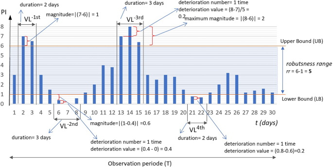
Vulnerability events for a performance indicator.
Magnitude-based metrics (MVM) quantify the total and maximum deviations (magnitude) of performance values \(x_t\) at time t below the lower bound LB (when defined) or exceeding the upper boundU UB. It is assumed that larger deviations indicate greater vulnerability. This metric reflects the hazard level associated with vulnerability impact. The magnitude value at time t ( \(MV_t\) ) is defined as the absolute difference between the value \(x_t\) and either the upper or lower bound (see Eq. 2). The total magnitude (MVM1) represents the overall impact of performance deviations (see Eq. 3), whereas the maximum magnitude (MVM2) reflects the worst-case performance (see Eq. 4).
$$\begin{aligned} MV_t = {\left\{ \begin{array}{ll} |x_t-UB|, & if \ UB \, exist \ and \ x_t > UB \\ |x_t-LB|, & if \ LB \, exist \ and \ x_t
(2)
$$\begin{aligned} MVM1 = \sum _{t \in T} MV_{t} \end{aligned}$$
(3)
$$\begin{aligned} MVM2 = \max {(MV_t)} \end{aligned}$$
(4)
Figure 4 illustrates:
\(MVM1 = 1 + 0.5 + 0.6 + 1 + 0.2 + 1 + 2 + 0.5 + 0.2 + 0.4 = 7.4\)
\(MVM2 = 2\)
Duration-based metrics (DVM) measure the total duration (DVM1) and the longest duration (DVM2) for which the performance value \(x_t\) remains outside the specified bounds of the robustness range. The duration of each out-of-range interval, \(\Delta t_{i}\), denotes the time span between two consecutive observation points t while the performance remains outside the specified bounds of the robustness range. A higher DVM indicates that the system is more fragile. The interval is calculated in Eq. (5). The total duration (DVM1) and the longest duration (DVM2) are represented in Eqs. (6) and (7), respectively.
$$\begin{aligned} \Delta t_{i} = t_{end,i} – t_{start,i} + 1 \end{aligned}$$
(5)
$$\begin{aligned} DVM1 = \sum _{i=1}^{n} \Delta t_{i} \end{aligned}$$
(6)
$$\begin{aligned} DVM2 = \max {\Delta t_{i}} \end{aligned}$$
(7)
Figure 4 shows that performance stays outside the bounds from t=2 to t=3 and then again from points t=6 to t=8, so the duration \(\Delta t_{1}\) is 2 days and \(\Delta t_{2}\) is 3 days, respectively. Then DVM1 and DVM2:
\(DVM1 = 2 + 3 + 3 + 2 = 10 \, days\)
\(DVM2 = 3 \, days\)
The Frequency-based Metric (FVM) counts the number of distinct episodes where the performance value lies outside the expected range boundaries during the observation period T. Each episode may span multiple consecutive time points but is counted as a single occurrence (see Eq. 8).
$$\begin{aligned} FVM1 = \sum _{t \in T} 1 (VL_{t} = 1 \, and \, VL_{t-1} = 0) \end{aligned}$$
(8)
Figure 4 illustrates that FVM1, the frequency of vulnerable conditions, occurs four times: twice below the lower bound and twice above the upper bound.
Deterioration-based metrics (DTM) count the condition when the performance value \(x_t\) remains outside the defined robustness boundaries and shows no improvement toward recovery but instead continues to deteriorate. This metric represents quantifying the severity of vulnerability. Equation (9) defines a condition when a system deteriorates. Equation (10) denotes the magnitude of deterioration at time t.
$$\begin{aligned} \begin{aligned} DT_t&= {\left\{ \begin{array}{ll} 1, & \text {if } \left[ \begin{array}{l} x_t UB \text { and } x_t – x_{t-1} > 0 \end{array} \right] \\ 0, & \text {otherwise} \end{array}\right. } \\&= {\left\{ \begin{array}{ll} 1, & \text {if } \bigl ( x_t UB \wedge x_t – x_{t-1} > 0 \bigr ),\\ 0, & \text {otherwise}. \end{array}\right. } \end{aligned} \end{aligned}$$
(9)
$$\begin{aligned} d_t = |x_t – x_{t-1} |,\ \text {if } \left[ \begin{array}{l} x_t UB \text { and } x_t – x_{t-1} > 0 \end{array} \right] \end{aligned}$$
(10)
Equation (11) define the total deterioration magnitude (DTM1). DTM1 represents the accumulated magnitude by which performance continues to deviate further away from the expected range during periods of vulnerability. It is computed as the sum of absolute differences between consecutive performance values when such values lie outside the robustness range and exhibit a deteriorating trend.
$$\begin{aligned} \begin{aligned} DTM1&= \sum _{t=2}^{T} \Bigl [ \textbf{1}\bigl ( x_t UB \wedge (x_t – x_{t-1})> 0 \bigr ) \cdot d_t \Bigr ] \\&= \sum _{t=2}^{T} \Bigl [ \textbf{1}\bigl ( x_t UB \wedge (x_t – x_{t-1}) > 0 \bigr ) \cdot |x_t – x_{t-1} |\Bigr ]. \end{aligned} \end{aligned}$$
(11)
Equations (12) define the number of deterioration occurrences (DTM2). DTM2 quantifies how many times performance begins to deteriorate further outside the robustness range across the observation period. Each occurrence signals a new episode of vulnerability intensification.
$$\begin{aligned} \begin{aligned} DTM2&= \sum _{t=2}^{T} \textbf{1}\bigl ( DT_t = 1 \wedge DT_{t-1} = 0 \bigr ) \\&= \sum _{t=2}^{T} \textbf{1}\Bigl ( \bigl ( x_t UB \wedge (x_t – x_{t-1}) > 0 \bigr ) \wedge \bigl ( DT_{t-1} = 0 \bigr ) \Bigr ) \end{aligned} \end{aligned}$$
(12)
Figure 4 illustrates that DTM2 occurs three times: twice below the lower bound and once above the upper bound.
Characteristic-based vulnerability metrics
System characteristics encompass internal preconditions (driver factors) and external exposure factors, both potentially influencing system vulnerability as defined in the model framework. Internal preconditions include attributes such as the number of available cabinets, the distance to the nearest neighboring station, the daily number of customers swapping batteries below the standard state-of-charge (SoC) threshold, and the number of users utilizing the station for private battery charging. In contrast, external exposure factors such as operational disruptions and environmental hazards, e.g., flooding.
Characteristic-based vulnerability metrics are computed via two methods: median absolute deviation (MAD) and static feature value ( \(x_{T}\) ). Static feature ( \(x_{T}\) ) is a value of an attribute from the driver or exposure factor that remains constant over the observation period. Examples of static features include the number of cabinets, distance to the nearest station, flood hazard indices, and monthly disruption counts. The values distinguish station profiles and potentially influence performance.
Conversely, process-related variables such as battery swap time, private charging duration, and customer inter-arrival times are evaluated using Median Absolute Deviation (MAD), as they typically exhibit temporal variation. MAD (Eq. 13) is preferred over the mean due to its robustness to non-normal distributions, making it more suitable for real-world data. It captures the variability in characteristic indicators over time, where higher variability may reflect a greater level of system vulnerability.
$$\begin{aligned} MAD = Median(|x – median(X)|) \end{aligned}$$
(13)
Scaling method
The scaling (normalization) method is performed to reconcile differences in scale and units across variables. A min–max scaling approach is used to map values into the [0,1] interval, with scaling direction determined by the metric orientation-either larger-is-more-vulnerable (LV), where higher values imply greater vulnerability, or smaller-is-more-vulnerable (SV), where lower values indicate higher vulnerability. As shown in Eq. (14), this ensures that normalized metrics near 1 correspond to high vulnerability levels.
$$\begin{aligned} MinMaxScale(x) = {\left\{ \begin{array}{ll} \frac{x-min[X]}{max[X]-min[X]}, if \, LV \\ \frac{max[X]-x}{max[X]-min[X]}, if \, SV \end{array}\right. } \end{aligned}$$
(14)
Vulnerability scoring formulation
The previous section established metrics for outcome vulnerability (i.e., performance) employing MVM, DVM, FVM, and DTM, and characteristics vulnerability using either MAD values or static feature values. The next section describes how these metrics are formulated to derive vulnerability scores for each battery swapping and charging station.
Consider a performance indicator used as an outcome-based vulnerability attribute. The performance indicator values are used to calculate vulnerability using outcome-based metrics such as MVM, DVM, FVM, and DTM, which are aggregated into the Performance Vulnerability Indicator (PVI). The outcome-based vulnerability score (OVIs) for a station s is computed as the average of the PVI metrics (Eq. 15a), where each \(PVI_{i,s}\) represents the aggregated values of the MVM, DVM, FVM, and DTM metrics for \(PVI_{i}\) at station s (Eq. 15b).
Similarly, let a driver factor and an exposure factor represent attributes of characteristic-based vulnerability. The characteristic-based vulnerability score (CVI) for a station s is calculated as the sum of the values from the vulnerability driver factor metric (VDF) and the vulnerability exposure factor metric (VEF) (Eq. 16a). The \(VDF_{s}\) is defined as the average of the vulnerability driver factors at a station s (Eq. 16b), while the \(VEF_{s}\) is computed as the average of the vulnerability exposure factors at a station s (Eq. 16c).
Finally, the vulnerability score for a station (Eq. 17) is obtained by aggregating the OVIs and CVIs, where the CVIs comprise the summed values of VDFs and VEFs (Table 1).
$$\begin{aligned} OVI_{s}&= \sum _{i=1}^{I} \frac{PVI_{i,s}}{I}, \forall \, s \in S \end{aligned}$$
(15a)
$$\begin{aligned} PVI_{i,s}&= (MVM1+MVM2+DVM1+DVM2+FVM1+DTM1+DTM2)/7 , \forall \, i \in I\, , \, s \in S \end{aligned}$$
(15b)
$$\begin{aligned} CVI_{s}&= VDF_{s} + VEF_{s} , \forall \, s \in S \end{aligned}$$
(16a)
$$\begin{aligned} VDF_{s}&= \sum _{j=1}^{J} \frac{VDF_{j,s}}{J}, \forall \, s \in S \end{aligned}$$
(16b)
$$\begin{aligned} VEF_{s}&= \sum _{k=1}^{K} \frac{VEF_{k,s}}{K}, \forall \, s \in S \end{aligned}$$
(16c)
$$\begin{aligned} \begin{aligned} VI_{s}&= OVI_{s} + CVI_{s}, \forall \, s \in S \\&= OVI_{s} + VDF_{s} + VEF_{s} , \forall \, s \in S \\&= \sum _{i=1}^{I} \frac{PVI_{i,s}}{I} + \sum _{j=1}^{J} \frac{VDF_{j,s}}{J} + \sum _{k=1}^{K} \frac{VEF_{k,s}}{K} , \forall \, s \in S \end{aligned} \end{aligned}$$
(17)
Table 1 Notation and Description.Performance vulnerability indicator (PVI), vulnerability driver factor (VDF) and vulnerability exposure factor (VEF)
A performance vulnerability indicator (PVI) refers to a set of system performance variables used to characterize vulnerability conditions, particularly when the performance values fall outside the expected or acceptable range. Outcome-based vulnerability metrics are applied to PVI to quantitatively assess the system’s level of vulnerability.
As outlined in the subsection Proposed Vulnerability Concept, two key terms are introduced: internal preconditions (driver factors) and exposure factors. In the following discussions, these terms will be referred to as the Vulnerability Driver Factor (VDF) and the Vulnerability Exposure Factor (VEF), respectively. Metrics such as MAD and static features (xT) are applied to the VDF and VEF, as will be elaborated in the following sections.
This section introduces some indicators of PVI, VDF, and VEF, in Tables 2, 3, and 4. The indicators or factors are adopted from prior studies such as those on manufacturing systems, logistics, and warehousing35,40,45,54, battery charging infrastructure20,38,55,56, battery storage systems57, and the British Standard – Maintenance Key Performance Indicators58. The selection of indicators and factors introduced in Tables 2 through 4 is limited by the scope of attributes available in the dataset obtained from an EM-BSCS service provider in Jakarta59.
Table 2 presents three examples of performance vulnerability indicators (PVIi), one of which is battery swapping throughput ( \(PVI_{1}\) ). Throughput may serve as a basis for station closure decisions when the value is critically low55. Throughput data, combined with the state of charge (SoC) of swapped batteries, can be used to estimate daily electricity consumption (kWh), which may design incentive schemes for users swapping batteries above a specific SoC threshold. Additionally, throughput can be used to calculate station occupancy38. Similarly, the second indicator ( \(PVI_{2}\) ) may capture battery utilization diversity, measured as the ratio of unique batteries ( \(PVI_{2}\) ) to swapping throughput ( \(PVI_{1}\) ). A higher ratio suggests lower vulnerability by reducing the risk of accelerated battery degradation.
Characteristic-based vulnerability variables include several driver and exposure factors, as presented in Tables 3 and 4. These factors may vary depending on system context and data availability. The state of charge (SoC) is an example of a driver factor, as frequent battery swaps at low SoC levels can reduce battery availability and accelerate degradation, thereby increasing EM-BSCS vulnerability. The median absolute deviation (MAD) of the SoC at each station is used as input for vulnerability scoring. Meanwhile, variables such as flood index and distance to the nearest station are considered static features ( \(x_{T}\) ), as they remain relatively stable over observation periods. Definitions and measurement methods for all factors are provided in Tables 3 and 4.
Table 2 The performance vulnerability indicators.Table 3 The vulnerability driver factors.Table 4 The vulnerability exposure factors.Fig. 5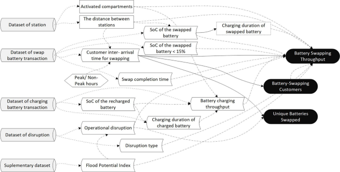
The relation scheme of PVI, VDF and VEF.
Figure 5 illustrates a relationship between the driver and exposure factors, which are assumed to affect the outcomes of the battery swapping and charging operations.


")